Andy’s Neural Works

Author: Andrew Della Vecchia

Date: 02/20/2023

Foreword

This post references a famous (and trendy) math problem that has yet to be solved. This should not deter anyone from trying and experimenting on their own. It is quite possible that your own unique view of the problem would bring new possibilities for a solution.

I often wonder what would happen if people studied a topic but did not receive any sort of degree, certificate, or badge. Would people still study it? Is a study only “worth it” if you get a gem to put in you crown? Would only those with true interest in the field pursue it further than the basics?

Everyone should take some confidence in their own abilities to learn on their own. Everyone should also realize that communication of success, failure, and general queries are a foundation of humanity. We can learn on our own but what is it to keep the treasure of discovery such a secret? Do not fear collaboration. True, there are destructive persons just waiting to be destructive. I believe you will find that there are also many more constructive persons. Be brave and confident even if you fail. You are always learning if you at least try.

My advice for everyone will always be to explore their educational interests even if it is simply a matter of reading a book. Mathematics is no different except you must practice to get good at it. Do not forget the roll of brown paper for your solutions.

Introduction to Analysis Goals

There is a well-known problem in the field of mathematics known as the Collatz Conjecture¹. It is studied vigorously. Despite those that say, “I solved it,” it remains unsolved. Still, there are those that chip away at it and discover a new way to look at it^{2, 3}.

This analysis is not a solution to the Conjecture. I would not be so bold. Sorry to disappoint you if you are looking for a solution. This is more of an exercise in abstract thinking and hope that someone out there will find it useful.

I was thinking about this problem in terms of being a task given to a data analyst. What if someone dropped a set of numbers on your desk, told you about the basics behind how they were generated, and let you go to study it. What could you come up with using a blank slate approach?

When I first saw the plots of how the sequences form a tree structure, I immediately thought of how this looks like a social network or maybe the way a database index is built. The way the numbers ebb and flow and create connections to a single actor reminds me of a big, directed graph. If each node is thought of as an actor in a network, the possibility of interesting analysis can be done. 

With the thought that this is a social network, can the process be considered as a way to create a communication web? What network gets developed and is it self-organized?

The approach to this exercise will be to:

• Review the look of each sequence and overall set built by using Julia⁴.
• Build basic stats on the set.
• Build a directed graph.
• Gain an understanding of the graph basics.
• Determine any cores that may exist.
• See if communities form.
• Determine distance measures.
• Determine interconnectedness of the vertices.
• Determine the measures of centrality.
• Discuss any conclusions.
• Form follow-up possibilities.

All these analysis components should provide a good exercise for the mind as well as a base for further efforts.

Overview of the Collatz Conjecture (aka 3n+1 Problem)

In 1937, mathematician Lothar Collatz proposed on a number sequence that follows a simple function that reacts on if the integer input is odd or even. If the input is even, the function would take the input and divide by 2. If odd, the function would multiple the input by 3 and add 1. That returned value is then used as a recursive feed into the same function.

This all sounds very simple on a surface level. It seems like a basic problem. The curious part deals with tracking the sequence as it progresses. What is observed is that the sequence seems to always end at 1. After 1, the sequence goes into a cycle where it goes up in value and then decays back down. Ultimately, it seems, the sequence returns to 1 again and again. This is referred to as a hailstone sequence since it is like physical hail that goes up and down till physical features bring it down to the ground. The question you should be asking is what starting value, or seed, can be used that will avoid sequencing to a 1?

Step back and do some historical reading. Such a simple problem should have been solved by now? No, it has not, despite many attempts. In fact, it has been stated that the math to create a solution has not been discovered yet.

Why study it, then?

The allure is that maybe you will be “the one” who solves it with some new form of math (or you just have the correct view to find a failing point). There is usefulness beyond proving whether it is valid or not. Looking at the sequence, plots, or abstract views, could there be something in nature that follows this pattern? Maybe, if matched properly, there is an application yet to be discovered which could create inventions to benefit humanity? Maybe a new way to organize communication networks? How about a new type of indexing strategy for structures? Possibilities always exist to improve the world around you. What is stopping you?

Code Overview

Why Julia Programming Language?

I will admit that I started this effort using R and Python with igraph. They are both useful languages and igraph is powerful in social network analysis. The issue is that performance of those languages is not that good in generating large sets. This causes simple logic changes to become more annoyance and deter from the excitement of the moment.

Having heard that the Julia Programming Language⁵ has higher performance that comes close to C, my curiosity got the better of me. Out of that interest, I decided to use the language. My results were positive. I could generate full sets in a fraction of the time. This made it easier to adjust and adapt alterations. I will say there are some issues found with libraries that are not as mature as the competition. I might have to write a separate article about those findings.

Functions to Generate Collatz Set

When coding the sequence, I wanted to be able to create an individual sequence directly from Julia’s REPL (acronym for Read-Eval-Print-Loop which is a form of interactive terminal). I came up with the following functions to meet this requirement:

Functions to Generate Graph using JuliaGraphs from Collatz Set

Generating a graph in Julia is straightforward if everything would be sequential. In this case, I am dealing with gaps in the sequence as well as overlaps. That requires converting the hailstone sequence to its vertex index in the graph.

Limitations Found

The core Julia Programming Language is well thought out. It contains the parts that make analysis straightforward to execute. Some similarity to Python is present along with additional simplicity. I find the package manager to be usually easy, but some install issues did occur. That required a bit of Internet research to correct.

At the beginning of the effort, I reviewed JuliaGraphs. It did not seem like it would have everything needed. I thought of using the Python interface in Julia for igraph (since Julia has some support for Python Packages). I might give it another go later down the road but the results were filled with many errors. JuliaGraphs would have to do for this effort.

JuliaGraphs by itself does support many features. Still, you can see how support and time has made igraph so powerful. I would think given some renewed interest; you might see an igraph interface ported to Julia (I believe there is an area in GitHub for this⁶).

Parameters

The set will contain seed sequences from 1 to 10,000. That is a far cry from the largest numbers ever tested. It is a good set for this purpose. I am approaching this as a techno-social network which makes 10K seed values a healthy number for our exercise

Exploratory Data Analysis (EDA)

I will now review some of the resultant data. Again, think of this as a standard data analysis effort. There is a general understanding of where the source comes from but what can be seen out of it?

Reviewing a few sequences

The first step after executing the generation process is to review some of the set visually. This will give a more “hands-on” grasp of the set. This is a list of the first 15 records in the set:

julia> cc_complete_set[1:15]
15-element Vector{Any}:
 [1]
 [2, 1]
 [3, 10, 5, 16, 8, 4, 2, 1]
 [4, 2, 1]
 [5, 16, 8, 4, 2, 1]
 [6, 3, 10, 5, 16, 8, 4, 2, 1]
 [7, 22, 11, 34, 17, 52, 26, 13, 40, 20, 10, 5, 16, 8, 4, 2, 1]
 [8, 4, 2, 1]
 [9, 28, 14, 7, 22, 11, 34, 17, 52, 26, 13, 40, 20, 10, 5, 16, 8, 4, 2, 1]
 [10, 5, 16, 8, 4, 2, 1]
 [11, 34, 17, 52, 26, 13, 40, 20, 10, 5, 16, 8, 4, 2, 1]
 [12, 6, 3, 10, 5, 16, 8, 4, 2, 1]
 [13, 40, 20, 10, 5, 16, 8, 4, 2, 1]
 [14, 7, 22, 11, 34, 17, 52, 26, 13, 40, 20, 10, 5, 16, 8, 4, 2, 1]
 [15, 46, 23, 70, 35, 106, 53, 160, 80, 40, 20, 10, 5, 16, 8, 4, 2, 1]

This all seems to follow through with what is expected. The seed values are present as is the hailstone sequence back to 1. Note that the first sequence is simply 1 as a point of reference since the sequence enters into an infinite loop and needs to be stopped manually.

Checking the set for missing values, none are found:

julia> findfirst(isequal(missing), cc_complete_set)

julia>

Basic Statistics

If the set is flattened out from an array of arrays, the describe function in Julia can be used to get the basic summary values:

julia> describe(cc_complete_set_flattened)
Summary Stats:
Length:         859666
Missing Count:  0
Mean:           7338.911652
Minimum:        1.000000
1st Quartile:   106.000000
Median:         592.000000
3rd Quartile:   2657.000000
Maximum:        27114424.000000
Type:           Int64

Reviewing the descriptive, the range is fairly wide. Finding the mode, Actor 1 is determined:

julia> mode(cc_complete_set_flattened)
1

A variable was set during our calculation for the standard deviation:

julia> set_std
91372.68714426944

That is standard deviation seems reasonable given the other metrics. Skew is notable. Again, I am taking a different approach when looking at the set.

Test for normality:

julia> using Pingouin

julia> Pingouin.normality(cc_complete_set_flattened)
[WARN] x contains more than 5000 samples. The test might be incorrect. Warning: p-value may be unreliable for samples larger than 5000 points
└ @ Pingouin ~/.julia/packages/Pingouin/L0EE5/src/_shapiro.jl:185
1×3 DataFrame
 Row │ W          pval          normal 
     │ Float64    Float64       Bool   
─────┼─────────────────────────────────
   1 │ 0.0351029  9.98949e-235   false

Interesting that it warns of issue with the test for large sample size. When digging through the documentation, there is a reference to Wikipedia on Shapiro-Wilks:

“Like most statistical significance tests, if the sample size is sufficiently large this test may detect even trivial departures from the null hypothesis (i.e., although there may be some statistically significant effect, it may be too small to be of any practical significance); thus, additional investigation of the effect size is typically advisable, e.g., a Q–Q plot in this case.”⁷

Running through the Q-Q Plot, I can see the cause for concern with normality:

That certainly looks different and against what would be expected as normal data.

Continuing with the approach, determine how many times are actors/nodes repeated in the complete set. Fortunately, the freqtable function makes this direct:

julia> sort(freqtable(cc_complete_set_flattened), rev=true)
21664-element Named Vector{Int64}
Dim1     │ 
─────────┼──────
1        │ 10000
2        │  9999
4        │  9998
8        │  9997
16       │  9996
5        │  9400
⋮              ⋮
12050854 │     1
13557212 │     1
15251866 │     1
18076282 │     1
22877800 │     1
27114424 │     1

Plotting the freqtable (sorted) and review:

Narrow range of numbers gets higher counts (removing the top 10 and the bottom tail). Reviewing a closer look:

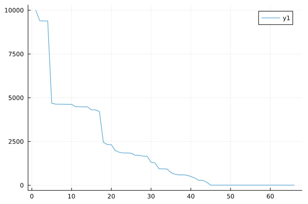
Looks like there is a core network of actors as seen by the large drop off upfront then the long tail at single networked players after.

Now reviewing the individual set lengths:

Interesting spread.

Reviewing the overall flow of average length increase of the set:

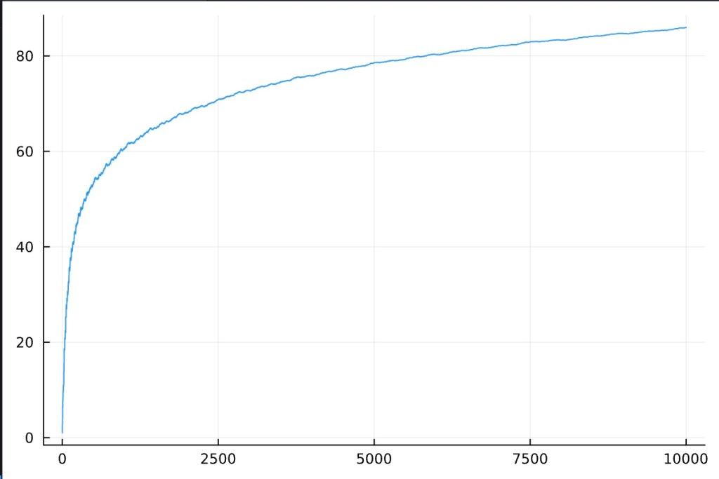
This is logarithmic looking. It is almost a bit of an art form in the way it smooths out over increased iterations.

Here is a plot of how the hailstone sequences look on top of each other. Notice the peaks up front then the tail.

For future effort, how far could this maximum be pushed on simple hardware?

Looking directly at the sequence means:

Means have some peaks here and there with a large spike at the high end. I expected it to be a bit higher but that could be due to the decay to 1 that happens consistently.

Consider what has been discovered so far. Again, use the idea that this is a techno-social network being built. It grows over time. As it does, what happens to the core players. Do communities form in other pockets? How do those that are periphery players become more established?

Running through the more standard approaches of reviewing data in different views, there is one item that stands out. As the set grows, the key actors become stronger in the network. This is due to the nature of how the hailstone sequence creates connections. It should be considered that the outer actors in elements mature over time into more solid connections. It is possible that all actors, even those with only single connections become critical players as growth of the network occurs.

Social Network Analysis (SNA)

Graph Rules

Here are the “givens” to be followed for building the base graph:

• Directed network.
• All vertexes represent as a single actor.
• There are no isolates.
• Edges are built once (i.e. duplicates are not considered) and in-order of discovery.
• No weights are given at this time. For future thought, possible base a weight on number of times the vertex is connected by new sequences other than itself.

After complete, here is a full plot using JuliaGraphs:

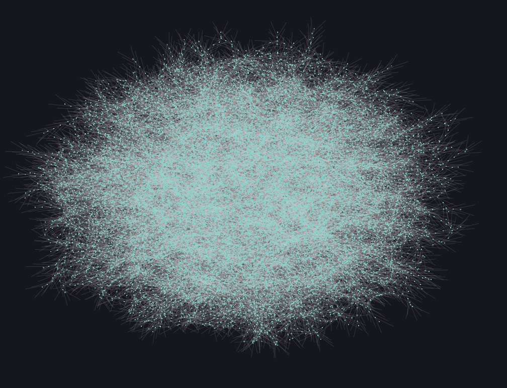
This is quite a complex and large graph. This creates a rather large hurdle with visual inspection even when scaling nodes (i.e. not quite easy to handle).

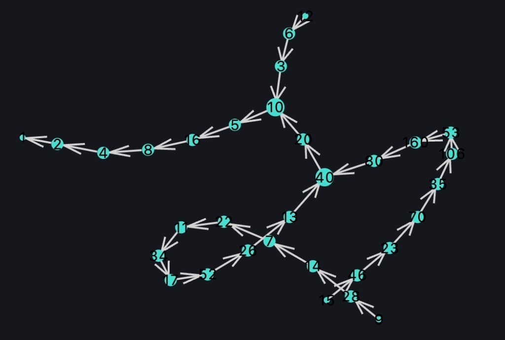
For reference only, the following is a reduced set for visualization purposes. The future sections will use a subsection for visual analysis only.

Graph basics

Here are the number of vertices:

nv = Graphs.nv(g)
julia> nv
21664

Here are the number of edges:

ne = Graphs.ne(g)
julia> ne
21663

This might seem average in efficiency in terms of vertices to edges. Further analysis is necessary here.

Cores

cores = Graphs.core_number(g)
julia> unique(cores)
1-element Vector{Int64}:
 1

Only 1 core exists. That is a noted as an area of interest for further investigation.

Community Measures

Running a quick calculation on clustering coefficient⁸ to determine community measure:

gclust = Graphs.global_clustering_coefficient(g)
julia> gclust
0.0

What this tells me is that there are no triplets in the network. Again, this is a directed network with pathways always directed to Actor 1.

Distances

Center

julia> ctr
21664-element Vector{Int64}:
     1
     2
     3
     4
     5
     6
     7
     ⋮
 21658
 21659
 21660
 21661
 21662
 21663
 21664

No differences to determine a true center are detected but what does that mean for our measures of centrality?

Diameter

julia> dia
9223372036854775807

Large value is noted which raises a question about its validity. This might be a result of some side-effects of having an end-to-end directed network.

Interconnectedness

den = Graphs.density(g)
avg_deg = mean(Graphs.degree(g))
avg_indeg = mean(Graphs.indegree(g))
avg_outdeg = mean(Graphs.outdegree(g))
min_deg = Graphs.δ(g)
min_indeg = Graphs.δin(g)
min_outdeg = Graphs.δout(g)
max_deg = Graphs.Δ(g)
max_indeg = Graphs.Δin(g)
max_outdeg = Graphs.Δout(g)

julia> den
4.615952732644018e-5

julia> avg_deg
1.999907680945347

julia> min_deg
1

julia> max_deg
3

This is interesting and further thought is needed for understanding. You can have one sequence where 3 goes to 10 as well as another sequence where 20 goes to 10. Finally, 10 goes to 5 and so on. That increases the degrees. How large of a set is needed to go above 3?

Looking further at in/out degree:

julia> avg_indeg
0.9999538404726735

julia> min_indeg
0

julia> max_outdeg
1

julia> avg_outdeg
0.9999538404726735

julia> max_outdeg
1

julia> min_oudeg
0

There are no extremes noted that are not expected.

Measures of Centrality⁹

For each centrality measure, the process executes the calculation with Julia Graphs’ built-in functions. Then, the results are sorted to bring the highest values to the top. The results are then filtered to gain the greatest and least 15 of the entire network.

In each section, I will also take a small subsection of the graph for visual analysis. This is done since trying to review the entire graph would be difficult for visual inspection.

Note on values: In most cases, the centrality measures that are reported go from 0 to 1 rather than whole numbers. For further definition as to how Julia calculations are done, please read through the system documentation references.

Degree Centrality

The degree centrality values are defined by the number of links connected to each node. I will go further into in and out degree centrality in the following sections since this is a directed graph.

The following table will be used in the remaining sections. It contains a top 15 query of the graph (descending order) along with a bottom 15 query of the graph (ascending order).

Nodes with Greatest DC Values	Nodes with Least DC Values
10 16 22 28 34 40 46 52 58 64 70 76 82 88 94	1  5001  5004  5007  5010  5013  5016  5019  5022  5025  5028  5031  5034  5037  5040

Some of these values should be expected. 10 is an actor that ties together a common sequence. I also see 1 as the node with the least values which is a given since it is on the termination point of sequences. We also have other nodes with same or similar values (if curious, run the code in the appendix within Julia). These could be the input Actors.

Degree Centrality Visual Review of Subsection

If I add the degree centrality value as a scaling factor for the size of the node in the subsection graph, the following visual is developed.

You can see the beginning and termination points are much smaller than the rest. Toward the central points (ex: 10 and 40), the points get much larger. The remainder of the sequence remains relatively stagnant.

In-Degree Centrality

The values here are based on the number of links coming into a node. The node with higher indegree centrality values are the ones with higher counts of incoming links.

Nodes with Greatest IDC Values	Nodes with Least IDC Values
10 16 22 28 34 40 46 52 58 64 70 76 82 88 94	5001 5004 5007 5010 5013 5016 5019 5022 5025 5028 5031 5034 5037 5040 5043

The list does look quite similar to the previous measure. Actor 1 is missing from the list which means it is not on an extreme point in the network in terms of in-degree centrality. It is possible that a weighted graph would provide more interesting results.

In-Degree Centrality Visual Review of Subsection

Scaling the nodes using indegree centrality measures, the following visual is now presented.

All of the origination nodes are the smallest values. That makes sense since they only have outgoing links. You can see the central nodes that have the most links are once again being highlighted. The rest are consistent values.

Out-Degree Centrality

Out-degree centrality measures the nodes based on the outgoing links.

Nodes with Greatest ODC Values	Nodes with Least ODC Values
2 3 4 5 6 7 8 9 10 11 12 13 14 15 16	1 2 3 4 5 6 7 8 9 10 11 12 13 14 15

The interesting item seen in this listing is that Actor 1 is a standout. If you analyze the values, you will see most are the same and that results in the overlap between greatest and least ODC columns. That is also seen in the sequential nature of the results.

Out-Degree Centrality Visual Review of Subsection

Scaling the nodes using out-degree centrality measures, the following visual is now presented.

Visually, you see that the values are consistent except for Node 1. That is noticeable because it does not have any outgoing links.

Eigenvector Centrality

Eigenvector Centrality shows a deeper relationship with neighbors Unfortunately, this could not complete without errors. This might result from the nature of the graph as previously seen but I am going reserve final judgement in future efforts with different libraries.

Betweenness

Betweenness measures are very useful in our case (as you will see in the subsection plot). This measure shows the values on common, central pathways. The nodes with greatest betweenness tend to be on the quickest pathways.

Nodes with Greatest Betweenness Values	Nodes with Least Betweenness Values
274 412 310 137 206 155 364 466 103 182 233 91 700 526 350	1 5001 5004 5007 5010 5013 5016 5019 5022 5025 5028 5031 5034 5037 5040

Now I see some nodes standing out. These are the values that could play critical junction points. If this were a true social network, I would analyze these actors are points for information injection/extraction.

Betweenness Visual Review of Subsection

Scaling the nodes using betweenness measures, the following visual is now presented.

You can see those critical pathway points standing out. These seem to follow previous actors of note. There is also a build-up and decay effect from the outer edges to the terminating point. Again, these are the points of interest in usual social network analysis.

Closeness

Dealing with closeness is a bit odd with an open end-to-end directed graph. There are some standouts.

Nodes with Greatest Closeness Values	Nodes with Least Closeness Values
6171 18514 9257 27772 13886 6943 20830 10415 31246 15623 7963 46870 23435 23890 11945	1 2 4 8 16 5 32 10 64 3 20 21 128 6 40

There are certainly different actors in play at this measure. If you run through the code and look at the values, you will see most are similar till you get closer to Actor 1. That is where the communication ends so it is expected that the closeness values will drop off.

Closeness Visual Review of Subsection

Scaling the nodes using closeness measures, the following visual is now presented.

It is noted that the values are consistent from start till the movement gets close to the end point. Actors 4 & 2 set the trend while actor 1 is the expected, determined end point.

Observations From Exercise Results

This exercise set out to see what can be gained from viewing the Collatz Conjecture as a social network. Only a snapshot in time has been analyzed. Is it reasonable that time as a variable can cause this approach to drastically change as expansion takes place?

On a high-level view, I can think of external players as being almost compartmentalized. They are one-way inputs to the network where each actor after is a feed forward player (like a Domino Effect). Actors at the end are the information sink.

It is seen that the communication pathway does have central players. These, possibly, have been developed over time as more actors are added but the predictable nature is something to be considered for this protocol. What were once compartmentalized actors are now central players. It is as if there are maturation features to this approach.

Despite being focused on getting information from the external ends, I can see there is a trunk in the tree. Key actors are not merely in the center. What can be thought of as a chain of communication can be thought of as structurally elastic. If there would be expansion or contraction to the network, I would see similar central players being reactively strong. This would also be a weak point for injection/extraction of information. How would the network react if there were losses centrally located?

Next Steps

This exercise is a start. There are features that have been uncovered for further experimentation. Possibilities that I note for future efforts:

1. Using a more mature set of coding libraries would be worthwhile for exploration and confirmation of exercise results. I plan on following-through with igraph. I will consider R and Python for that aspect if efforts with Julia’s interface does not work out. Dive deeper into previous results using igraph.
2. Can an optimization of the network be done?
3. Will there be a way to bypass connections for performance?
4. What does this network look like over time as it expands?
5. Can I shrink/optimize the network without breaking the conjecture?
6. What happens to key players during major expansion
7. Weight algorithm should be applied to connections. Will this result in a balanced communication path?
8. Simulation of key actor removal
9. Efficiency improvements

Appendix

Code Listing

#----------------
# Date:    12/23/2022
# Title:   Collatz Conjecture Analysis with Julia
# Author:  Andrew Della Vecchia
# Purpose: Experiment for social-network analysis of Collatz Conjecture Sequences
#----------------

# Libraries
using Graphs, GraphPlot, StatsBase, StatsPlots, FreqTables, Printf

# Base rule of Collatz Conjecture
function cc_base(x)
    if x % 2 == 0
        return Int(x/2)
    else
        return 3*x+1
    end
end

# Generate Collatz Sequence based on seed
function cc_sequence(x)

    # Init
    n = x
    seq = [x]

    while n!=1
        n = cc_base(n)
        #print(n)
        push!(seq, n)
    end

    return seq
end

# Generate the entire Collatz Set based on seed parameters
function generate_cc_set(seed_start, seed_end)

    cc_full_set = []

    for i in seed_start:seed_end
        cc_seq = cc_sequence(i)
        push!(cc_full_set, cc_seq)
        #print(seq)
    end

    return cc_full_set

end

# Pass in original value and return the vertex index in a graph
function vertex_index(original_vertex, vertices)

    return findfirst(isequal(original_vertex), vertices)

end

# Develop unique list of vertices and sort it
function uvertices(cc_set)

    # Init
    unique_vertices = []

    # Go through all of the generated Collatz Sequence
    for cc_seq in cc_set

        # build out the graph components
        for cc_value in cc_seq

            # If the vertex is not capture in list to be graphed, capture it
            if !(cc_value in unique_vertices)
                push!(unique_vertices, cc_value)
            end

        end

    end

    # Do not forget to sort the value at the end
    return sort(unique_vertices)

end

# Generate edge list but ensure it is indexed to JuliaGraph expected indexing
function edges(cc_set, vertex_list)

    # Init
    all_edges = []

    # Go through all of the generated Collatz Sequence
    for cc_seq in cc_set

        # build out the graph components
        for i in eachindex(cc_seq)

            # Make sure you do not overflow the array
            if i < length(cc_seq)
                    
                #build out edge
                edge = [vertex_index(cc_seq[i], vertex_list), vertex_index(cc_seq[i+1], vertex_list)]

                # If Edge does not exist in list to be graphed, capture it
                if !(edge in all_edges)
                    push!(all_edges, edge)
                end

            end

        end

    end

    return all_edges

end

# Build out all of the graph components
function generate_graph(cc_set)

    # Generate indexed and sorted vertices list findfirst
    indexed_vertices = uvertices(cc_set)

    # Generate the edge list
    all_edges = edges(cc_set, indexed_vertices)

    # Develop directional graph
    g = SimpleDiGraph()

    add_vertices!(g, length(indexed_vertices))

    for e in all_edges
        add_edge!(g, e[1], e[2])
    end

    return g, indexed_vertices, all_edges

end

# Utility function to find value in a subsequences/array (example: find all sequences containing node 2)
function find_in_sub_array(v_find, prime_set)

    #Init
    ret_hits = []

    for seq in prime_set
        if !(findfirst(isequal(v_find), seq) == nothing)
            push!(ret_hits, seq)
        end
    end

    return ret_hits

end

# Generate the set
cc_complete_set = generate_cc_set(1, 10000)
cc_complete_set_flattened = [(cc_complete_set...)...]

# EDA
# Basic stats

# Max/Min
minv = findmin(cc_complete_set_flattened)[1]
maxv = findmax(cc_complete_set_flattened)[1]

#overall values
set_mean = mean(cc_complete_set_flattened)
set_std = std(cc_complete_set_flattened)
#describe(cc_complete_set_flattened)

counts(cc_complete_set_flattened) # show the counts/distribution (sort by counts)

# Find sequence length, total sequence length average across set, and std dev
set_means = []
set_sd = []
set_lengths = []
set_avg_lengths = []
p_sequence = plot(legend=false, xlabel = "Step #", ylabel = "Hailstone Value")

for seq in cc_complete_set

    push!(set_means, mean(seq))
    push!(set_sd, std(seq))

    l = length(seq)
    push!(set_lengths, l)
    push!(set_avg_lengths, mean(set_lengths))

#    @printf("sequence: %i, length: %i\n", seq[1], length(seq))

    #build out the plot show hailstone sequences
    plot!(p_sequence, 1:l, seq)

end

#plot out the lengths to show the grow/shrink effect
p_lengths = plot(set_lengths, xlabel = "Seed", ylabel = "Sequence Length", legend=false)

#see the lengths average out as set increases in size
p_avg_lengths = plot(eachindex(set_avg_lengths), set_avg_lengths, legend=false)


# Get a general feel for counts
sort(freqtable(cc_complete_set_flattened), rev=true)

# How many intersections in the network? How many times do things intersect (besides 16, 8, 4, 2, 1)
print(sort(freqtable(cc_complete_set_flattened), rev=true)[1:20])


# Generate the graph
g, vertex_list, edge_list = generate_graph(cc_complete_set)


#print(g)
#print(vertex_list)
#print(edge_list)

# Plot out the graph
#gplot(g, layout=random_layout, nodelabel = vertex_list)

# SNA

# Basics
# Number of components
nv = Graphs.nv(g)
ne = Graphs.ne(g)

# Cores
cores = Graphs.core_number(g)

# Community
gclust = Graphs.global_clustering_coefficient(g)
asty = Graphs.assortativity(g)

# Distance
ctr = Graphs.center(g)
dia = Graphs.diameter(g)
rad = Graphs.radius(g)

# Interconnectedness
den = Graphs.density(g)
avg_deg = mean(Graphs.degree(g))
avg_indeg = mean(Graphs.indegree(g))
avg_outdeg = mean(Graphs.outdegree(g))
min_deg = Graphs.δ(g)
min_indeg = Graphs.δin(g)
min_outdeg = Graphs.δout(g)
max_deg = Graphs.Δ(g)
max_indeg = Graphs.Δin(g)
max_outdeg = Graphs.Δout(g)

# Centrality
dc = Graphs.degree_centrality(g)
sort(dc, rev=true) #shows the sorting from greatest to smallest
dc_sortperm = sortperm(dc, rev=true)
dc_sorted_15 = vertex_list[dc_sortperm][1:15]

idc = Graphs.indegree_centrality(g)
idc_sortperm = sortperm(idc, rev=true)
idc_sorted_15 = vertex_list[idc_sortperm][1:15]

odc = Graphs.outdegree_centrality(g)
odc_sortperm = sortperm(odc, rev=true)
odc_sorted_15 = vertex_list[odc_sortperm][1:15]

bc = Graphs.betweenness_centrality(g)
bc_sortperm = sortperm(bc, rev=true)
bc_sorted_15 = vertex_list[bc_sortperm][1:15]

#ec = Graphs.eigenvector_centrality(g)
clc = Graphs.closeness_centrality(g) #, distmx=weights(g); normalize=true)
clc_sortperm = sortperm(clc, rev=true)
clc_sorted_15 = vertex_list[clc_sortperm][1:15]


#Graphs.dominating_set(g, DegreeDominatingSet()) # nothing conculsive

# See if network can be reduced
sg = Graphs.squash(g)
(g != sg) ? "Squashed is same" : "Squashed is different"

References

1. Weisstein, Eric W. “Collatz Problem.” From MathWorld–A Wolfram Web Resource. Wolfram MathWorld. Retrieved from: https://mathworld.wolfram.com/CollatzProblem.html
2. Tao, Terence. The Notorious Collatz conjecture. Retrieved from: https://terrytao.files.wordpress.com/2020/02/collatz.pdf
3. Hartnett, Kevin. Mathematician Proves Huge Result on ‘Dangerous’ Problem. Quanta Magazine. December 11, 2019. Retrieved from: https://www.quantamagazine.org/mathematician-proves-huge-result-on-dangerous-problem-20191211/
4. The Julia Programming Language. Retrieved From: https://julialang.org
5. Miller, Sandi. MIT-created programming language Julia 1.0 debuts. MIT Department of Mathematics. August 27, 2018. Retrieved from: https://news.mit.edu/2018/mit-developed-julia-programming-language-debuts-juliacon-0827
6. Julia interface to igraph. Edited: Jan 15, 2015. Retrieved from: https://github.com/igraph/igraph/wiki/Julia-interface-to-igraph
7. Wikipedia. Shapiro–Wilk test. Retrieved from: https://en.wikipedia.org/wiki/Shapiro–Wilk_test
8. GeeksForGeeks. Clustering Coefficient in Graph Theory. Retrieved from: https://www.geeksforgeeks.org/clustering-coefficient-graph-theory/
9. Disney, Andrew. Social network analysis 101: centrality measures explained. January 2, 2020. Retrieved from: https://cambridge-intelligence.com/keylines-faqs-social-network-analysis/