Andy’s Neural Works

Published on: November 29, 2023

Author: Andrew Della Vecchia

Introduction

In the previous parts of this series on randomness, I alluded to the thought that a pseudorandom number generator (PRNG) could be predetermined because it is not truly random. Now is the time to determine the truth to that statement. As in all good research efforts, we start by asking a question or stating an observation. For this research goal I ask, “can the output of a PRNG be known beforehand? If so, how easy is it to do so?”

My expected result is that it can be done. I don’t know how easy it will be to achieve. My hypothesis is that it would be a challenge on my laptop. There may be more to this than originally thought.

Please note that this article will focus on the experimentation. I will try to explain the process at each experiment starting point then discuss the results. If not directly available in the article text, code or links to any externally sourced code will be provided in the appendix as well as references.

Time to have some fun. There are different approaches we can take but let us start with the most simplistic approach. I do not expect good results there so I will use more finesse in the subsequent attempts.

As you read through these experiments, keep this very famous quote in your mind.

“Know the enemy and know yourself; in a hundred battles you will never be in peril. When you are ignorant of the enemy, but know yourself, your chances of winning or losing are equal. If ignorant both of your enemy and yourself, you are certain in every battle to be in peril.”

-Sun Tzu, The Art of War¹

Hunt the Seed

Recall that the process of generating a random number requires an initial value, the seed. From this single point, the entire sequence is generated. Remember that deterministic systems produce the same outputs for the same inputs.

In some cases, the seed is set. In other cases, the default value is chosen. For Mersenne Twister (MT)² and Python³, the default value is either the system time at execution or a value generated from the Operating System (OS). This makes the process of brute force methods an interesting challenge. For reference, here is the function signature and remarks for the seed defined in random.py⁴.

def seed(self, a=None, version=2):
        """Initialize internal state from a seed.

        The only supported seed types are None, int, float,
        str, bytes, and bytearray.

        None or no argument seeds from current time or from an operating
        system specific randomness source if available.

        If *a* is an int, all bits are used.

        For version 2 (the default), all of the bits are used if *a* is a str,
        bytes, or bytearray.  For version 1 (provided for reproducing random
        sequences from older versions of Python), the algorithm for str and
        bytes generates a narrower range of seeds.

        """

This brings up a point here. Do you know the random number algorithm being used for that sequence you are looking to crack? Is it even a single algorithm or is there a bit of cleverness that switches around the algorithm to create confusion. This discussion could go on in many different directions. For purposes of keeping the exploration on track, I will define the algorithm as the Mersenne Twister.

Brute Force Approach

This technique is really a tedious approach unless you happen to be lucky. In the most extreme case, the idea is to start at a low point for a seed, generate a random number sequence and see if it matches. If it does not match, increment the seed by a value then generate another sequence to see if it matches. This keeps on moving forward till a match happens or you just get tired of burning through CPU cycles and electricity.

Here is one possible approach using Python:

# Init values
limit_attempts = 100000000000
count_attempts = 0
hit_found = False
seeds = range(limit_attempts)
rn_to_find = 0.8852272812021744 # this is the value trying to be generated (floating point number is picked to demonstrate difficulty)

# Iterate until a hit is found or you exhaust patience
while hit_found == False and count_attempts < limit_attempts:
    random.seed(seeds[count_attempts])
    rnd_value = random.random()
    hit_found = (rnd_value == rn_to_find)
    count_attempts += 1

# Show if the hit was found
print(f'hit_found: {hit_found}')
print(f'count_attempts: {count_attempts}')

If the target random number sequence is simple, you can eventually get a match. That is an unrealistic case, though. With most implementations, the idea is to create a very good random number and not one that can be guessed easily. Keep that in mind whenever coding with a PRNG.

I will alert you at this point that the particular developer might be choosing to use a random seed function (ex: os.urandom). In this case, a brute force approach would get tedious unless there is hefty set of processing resources available.

How would someone know at this point what to do? Consider thinking through the seed outside of a formula or a compounding of algorithms. Try to understand a seed that is chosen upfront. If you read through different research papers that show their code, you could very well see the seed is set to the same value. This is done for repeatable results generation. I am not a proponent of this approach outside of a study showing work. In other words, keep them guessing!

Uncover the System Time

What do you do with this information besides a basic loop that tries and tries? It is a good idea to get into the mind of the developer. Don’t go too deep. Some developers are a bit eccentric. What if the seed has some repeatable meaning to the developer? 

One item to consider is if the original developer decided to set the seed to system time. This is actually a common practice. It usually means an integer value representing time back to the Unix Epoch⁵. For those unaware, this value is the number of seconds going back to January 1, 1970 at 00:00:00 (midnight in Coordinated Universal Time). One method to try would be to set the seed to the time of generation and push forward from there. This could put the brute force approach into more of a directed force.

Here is an example of generating a seed in Python. This can be used instead of the previous seed.

seed_dt_string = '2023-11-25 14:05:00.000000'
seed_dt = dt.datetime.strptime(seed_dt_string, "%Y-%m-%d %H:%M:%S.%f")
seed_in = int(seed_dt.timestamp())
seeds = range(seed_in, seed_in + limit_attempts)

Note: One could also ignore using integer values and increment the time variable directly by parts of a second.

Does this really improve the approach? I would say it does, but it’s only one step above guessing.

Use a “Feel Good” Seed

In researching this article, I simply queried “popular seeds to use for a rng.” The number 42 is quickly returned from various web search engines. There it is in all its nuttiness. For the uninitiated, the number 42 is referenced in Douglas Adams’ Book, The Hitchhikers Guide to the Galaxy as the answer to the question of “Life, the Universe and Everything.”⁶ This seed value must be popular due to a psychological factor to prove one’s geek-cred. So, why not plug this number in and see what it generates?

import random
random.seed(42)
print(f'random number: {random.random()}')

Running this, we have 0.6394267984578837 as the random number.

I then tried several machines loaded with different versions of Python (even on an iPad). They all produced the same value when random() was called. This should warn us not to be too clever by half!

One interesting item is when I went back and tried in different languages. I tried in R and Julia with a seed of 42. They gave different results! Ah! That means to properly replicate the sequence, it is more than just the algorithm but the specific implementation of the algorithm.

With this result, we are getting more focused. A curious person could research a list of popular seeds as a base for analysis. That is a step better in this research but still far from intelligent.

Hunting with an AI Guide

Let’s take a break. I want to try out the approach that came out of the Microsoft Camp when visual analysis was done back in part 2. Bing’s AI Chat⁷ decided that it saw a pattern that looked like the rose plot where the formula given is r = sine(2*theta)). That is not difficult to generate using some code. Let’s look at the polar plot:

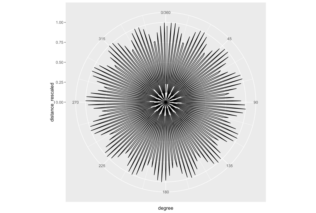
Even though there are similarities, doing comparisons with the underlying values show differences certainly exist. The distances are rescaled to go between 0 and 1.

mean(standard_rng$random_number[1:360] - pred.rose$distance_rescaled[1:360])
[1] -0.000132042

 max(standard_rng$random_number[1:360] - pred.rose$distance_rescaled[1:360])
[1] 0.958416

min(standard_rng$random_number[1:360] - pred.rose$distance_rescaled[1:360])
[1] -0.9687602

Maybe this could be used for approximation, but not for the exact matches I am trying to find. Even if I run a search to go through the entire set of random numbers, no match is found. This has been a fun exercise, but it is time to move on. Although a cool looking plot that raised an eyebrow, the results did not hit the target. Let us see if the values can be predicted with some learning algorithms.

Predictive Hunting

There is much said about the power of machine learning. We know that given enough historic data, the statistical models will be able to predict future values. There is always the question of accuracy. With a good RNG, prediction is not expected. It is something that needs to be tried.

Linear Model

This should be an easy experiment to do in R. I will use the previously generated sequence of numbers from part 2 of this series to make it more interesting. The model will be built using the first 100,000 rows of values as the training set. Again, this is due to hardware limitations. The fitting will use the random number value as the dependent variable and the row number as the independent variable.

Then, we will run a prediction and compare to the known values. I am not sure how much success is going to happen given there is not much of a linear pattern to the data.

Call:
lm(formula = random_number ~ ., data = standard_rng_train)

Residuals:
     Min       1Q   Median       3Q      Max 
-0.50085 -0.25099  0.00008  0.25190  0.50143 

Coefficients:
             Estimate Std. Error t value Pr(>|t|)    
(Intercept) 4.984e-01  1.828e-03 272.593   <2e-16 ***
rownumber   2.633e-08  3.167e-08   0.831    0.406    
---
Signif. codes:  0 ‘***’ 0.001 ‘**’ 0.01 ‘*’ 0.05 ‘.’ 0.1 ‘ ’ 1

Residual standard error: 0.2891 on 99998 degrees of freedom
Multiple R-squared:  6.914e-06,	Adjusted R-squared:  -3.086e-06 
F-statistic: 0.6914 on 1 and 99998 DF,  p-value: 0.4057

Not really seeing much of a joyous result. Let us review the plot (number of points reduced to 1000 values for clarity).

That plot really makes it look like the model is not going to work. The noisiness of those data is obvious. The middle point and straightness of the model indicates even distribution.  I will now run a prediction and see what happens.

Root Mean Squared Error of Predictions (RMSE): 0.4982152

R-Squared of Predictions: 0.02187228

The RMSE and R² do not indicate a good set of predictions out of the model. There was not a real linear layout to the values.

It can be said that using a linear model to do predictions on the random number sequence is not a valid approach. I did repeat the numbers using different samplings from the random number set. This did not change the results much at all.

I am not ready to give up on the use of predictive algorithms. What about more advanced learning models, such as a neural network? Is it possible there could be some interesting findings? Let us find out!

Long Short-Term Memory Model (LSTM)⁸

The idea of using a neural network is very enticing. Where a linear model works according to a specific fit, a neural network can be more flexible. There are various types of networks to pick from. Which one is best? If I were to go through each one, I probably would spend many days, if not weeks or months. Instead, I will rely on my readings where I found that using Long Short-Term Memory Model is very good at prediction with sequential data⁹. This is in-line with what is needed.

For this experiment, training data are needed to properly configure the network. This is going to be a straightforward sequence from the PRNG Mersenne Twister already developed in part 2 of this series. I will use Google Colab since Keras and Tensorflow setup is odd on the Apple M1 (lookup tensorflow-metal¹⁰). I will also, cautiously, ask Google Bard¹¹ for its view on how to build the LSTM layers since there are many ways this can be done. I will give Bing Chat a chance at it too. Even with those actors in the mix, I will do my best to keep it simple.

Here is the layout of the resulting model:

The training data set is composed of the first 80% of the 100K records previously discussed in the linear model approach. The test data are the remaining 20% of the 100K record set.

The training of the model is executed using the training data as input and output. This might seem odd at first. In practice, this is an autoencoding¹² technique. That is useful for this scenario where the sequence is noise.

Once the model is compiled, a prediction is run using the test data. Here are the resulting RMSE and R² of predicted and test values:

Root Mean Squared Error: 0.00011641125090193064

R-Squared: 0.9999998396304708 <- Strong correlation!

The results look very promising! Caution should be noted since the predictions are not a perfect match. Does this mean the algorithm is not valid for this application? Even though the model is an advanced design, there are differences to make it an imperfect match. Still, we should be encouraged by the results.

I will also state that the model layers are not perfectly configured. Honestly, there are better approaches than what I am using. That takes much more experimentation where others have had success.

If the goal is to get the exact number, it is not that easy to predict even with a learning model. I don’t take this as a failure. What if the goal was to get in the general neighborhood of the random number? Imagine a scenario where you need to predict the co-ordinates of some opposing force. You probably have previous history where it seems random. Having the exact co-ordinates would be ideal but an approximation would certainly be useful. This sounds like a good future experiment.

Hunt the Algorithm

The evidence generated so far shows how difficult random number prediction can be. The brute force approach that we explored first ended up being rudimentary. It is a guessing game that may never end. Trying to use social engineering techniques on the developer sounds like something out of a fantasy story. Predictive modeling is very interesting but did not give ideal results. There is potential in predictive modeling, but it requires more rigorous research. What to do now? Remember that quote at the beginning of this article about knowing the enemy? Think about that for a second.

How about reverse engineering the Mersenne Twister Algorithm itself? This has been done and it is a wonderful experiment. If you query for reverse engineering Mersenne Twister, you will see that it is very possible^{13, 14, 15, 16}. The idea is to take a sequence of random numbers from the PRNG and backfit using clever bitwise math.

To be exact, there needs to be 624, 32-bit wide values used. It is that size due to algorithm complexity and the impact on resource performance. A wider sequence could slow the system. During execution, a sequence of 624 numbers creates the internal state of the PRNG. This sequence is used to generate the next set of values during what is called the “twist” call. The process feeds the values forward to the next sequences.

If you can gather a consistent sequence, you would then have the internal state of the PRNG. In essence, you have enough data to build out the playbook used to generate subsequent sequences. At that point, you are victorious in your quest. 

Let’s give it a try. There are numerous sites on this approach. Implementations vary slightly but the underlying concept is the same. For this experiment, I made sure to pick a version that is built in Python¹⁷.

As is seen in the following output, this a bit too easy. After creating an instance of the predictor class, the required property is set to a series of 32-bit random numbers.

predictor = MT19937Predictor()
for _ in range(624):
	x = random.getrandbits(32)
	predictor.setrandbits(x, 32)

At this point, you can experiment to see if the random library output matches the predictor output.

print(random.getrandbits(32) == predictor.getrandbits(32))
print(random.random() == predictor.random())

These will both output “True.” As a final test, a shuffle is performed on the sequence:

a = list(range(100))
b = list(range(100))
random.shuffle(a)
predictor.shuffle(b)
print(a == b)

Again, a “True” is output which indicates success in replicating the internal state of the PRNG. This reverse-engineering is not only possible, but also quick. Compare this to the brute force approach, which can run on for hours and even days, to see the benefit of understanding algorithmic design.

With this success, we see the light at the end of the tunnel. All the experiments performed to this point have provided plenty of interesting results. I believe that many more experiments can be tried but enough has been discovered for a conclusion.

Conclusions

Reviewing the research question, “can the output of a PRNG be known beforehand,” we find that answer is a yes. There are different approaches that can be done with success.

At least, it is proven for the Mersenne Twister PRNG Algorithm. Can that be said for all PRNGs? I feel enough confidence now to say that answer is a yes.

How easy it is to predetermine the output varies. Some are very simplistic and might use social engineering skills, such as guessing or finding out a favorite number for the seed. Other approaches require digging deep and using a lot of processing time. Even if accomplished, those techniques are tedious.

The best technique is to be resourceful. In the case of Mersenne Twister, the internal workings are known. That gives a bit of an advantage to analyze the various working parts. If it were all unknown, reverse engineering the algorithm would be more challenging.

An item I left out would be to go into more aggressive aspects such as programming to the metal¹⁸. In other words, go right to the hardware addresses and get an output from the underlying circuitry. Anyone friendly with Assembler¹⁹ would certainly want to dive into that approach.

There are certainly many more aspects of RNGs to explore. Maybe you can do some of that exploration and share with everyone. Never be afraid to give simple exploration of technology a try. Start with the knowns, do research, and open one of the many code editors out there for anyone to try. You might be surprised with what you find inside that God-given brain of yours.

I do think I need to take a bit of break from the topic but will come back with a concluding article. There are some more experiments needed. Maybe, possibly, someday, I will even create my own RNG that will be useful to someone.

Thank you and have a great day!

Appendix

Code

The code provided here is in an AS-IS condition. Code is always in flux in order to experiment in many ways. Use at your own risk.

Rose Algorithm – R

# Title:      Exploration in Randomness – Part 3 - Rose Algorithm
# Author:     Andrew Della Vecchia (algorithm identified by Bing Chat)
# Purpose:.   This is used for RNG prediction experiments in article for Andrew's Folly (http://www.andrewsfolly.com)
# Conditions: AS-IS condition. This is completely experimental code with no guarantees.

# libraries
library(tidyverse)
library(scales)

# load the RNG output files
source_path <- '' # set to the path of the file contain the random numbers
standard_rng <- read_csv(file.path(source_path, 'standard_rng.csv'), col_names = 'random_number')

# create tibble using rose calculation (sine(2*theta))
pred.rose <- tibble(distance = sin(2*(1:360)), degree = 1:360, radians = (1:360) %% 360 * pi/ 180)
pred.rose <- pred.rose %>%
  mutate(distance_rescaled = rescale(distance))

# polar plot and scale value to 
pred.rose.polar_plot <- ggplot(pred.rose, aes(x=degree,  y=distance_rescaled)) +
  geom_line() +
  #  geom_point() +
  coord_polar() +
  scale_x_continuous(limits = c(0,360),
                     breaks = seq(0, 360, by = 45),
                     minor_breaks = seq(0, 360, by = 15)) +
  ylim(0, NA)

pred.rose.polar_plot

# determine the difference if we do not align at all
mean(standard_rng$random_number[1:360] - pred.rose$distance_rescaled[1:360])
max(standard_rng$random_number[1:360] - pred.rose$distance_rescaled[1:360])
min(standard_rng$random_number[1:360] - pred.rose$distance_rescaled[1:360])

# are there any cases where any RNG value is equal to the generate value from the rose model?
print(length(intersect(pred.rose$distance_rescaled, standard_rng$random_number)))

# no values match
# scale of numbers is different
# what if the values are rounded?
for (scale_value in 1:10) {
  
  distance_rescaled_rounded <- round(pred.rose$distance_rescaled, scale_value)
  random_number_rounded <- round(standard_rng$random_number, scale_value)
  
  print(length(intersect(distance_rescaled_rounded, random_number_rounded)))
  
}

Prediction with Linear Model – R

# Title:      Exploration in Randomness – Part 3 - Linear Model
# Author:     Andrew Della Vecchia (algorithm identified by Bing Chat)
# Purpose:  This is used for RNG prediction experiments in article for Andrew's Folly (http://www.andrewsfolly.com)
# Conditions: AS-IS condition. This is completely experimental code with no guarantees.

# libraries
library(tidyverse)
library(scales)
library(caret)

# load the RNG output files
source_path <- ' ' # set to the path of source file containing list of random numbers
standard_rng <- read_csv(file.path(source_path, 'standard_rng.csv'), col_names = 'random_number') # adjust as needed to file name

standard_rng <- standard_rng %>%
  mutate(rownumber=row_number())

split_index <- 100000

standard_rng_train <- standard_rng[1:split_index,]
standard_rng_test <- standard_rng[-split_index,] # Note: this gets adjusted as needed

rn.lm <- lm(random_number ~ ., standard_rng_train)

print(rn.lm)
summary(rn.lm)
#plot(rn.lm) # caution using this in low memory systems

prediction_seq <- list()
prediction_seq$rownumber <- seq(100001, 100010) # set to max length if brave

rn.pred <- predict(rn.lm, prediction_seq, interval = 'prediction')
rn.mse <- mean((rn.pred - standard_rng_test[1:length(rn.pred), ]$random_number)^2)
rn.rmse <- RMSE(rn.pred, standard_rng_test[1:length(rn.pred), ]$random_number)
rn.r2 <- R2(rn.pred, standard_rng_test[1:10,]$random_number)

Prediction with LSTM – Python

# Title: Exploration in Randomness – Part 3 – Predicting a random number with a LSTM
# Author: Numerous Sources (Bard, Bing, Stack Overflow, and more) and Andrew Della Vecchia
# Purpose: Experiment with LSTM. This is used for RNG experiments in article for Andrew's Folly (http://www.andrewsfolly.com)
# Conditions: only use in AS-IS condition. This is completely experimental code with no guarantees.

# imports/libraries
import numpy as np
from tensorflow.keras.models import Sequential
from tensorflow.keras.layers import LSTM, Dense
from google.colab import drive
import math
from sklearn.metrics import r2_score

# Read in the data from the previously generated file
drive.mount('/content/gdrive')
rng_data = np.genfromtxt('/content/gdrive/MyDrive/standard_rng_100K.csv', delimiter=',')
rng_data = rng_data.reshape(-1,1)

# split data into train and test sets
train_data = rng_data[:80000]
test_data = rng_data[80000:]

# Create the LSTM model
model = Sequential()
model.add(LSTM(50, return_sequences=True, input_shape=(train_data.shape[1], 1)))
model.add(LSTM(50))
model.add(Dense(1))

# Compile the model
model.compile(loss='mean_squared_error', optimizer='adam')

# Train the model
model.fit(train_data, train_data, epochs=10, batch_size=32)

# Make predictions
test_data_predictions = model.predict(test_data)

rmse = math.sqrt(np.mean((test_data_predictions - test_data)**2))
print(f'Root Mean Squared Error: {rmse}')

r2 = r2_score(test_data_predictions, test_data)
print(f'R-Squared: {r2}')

References

[1] Sun Tzu. The Art of War. January 1, 401. Retrieved from Good Reads: https://www.goodreads.com/quotes/730164-know-the-enemy-and-know-yourself-in-a-hundred-battles

[2] M. Matsumoto and T. Nishimura, “Mersenne Twister: A 623-dimensionally equidistributed uniform pseudorandom number generator”, ACM Transactions on Modeling and Computer Simulation Vol. 8, No. 1, January pp.3–30 1998. Retrieved from: http://www.math.sci.hiroshima-u.ac.jp/m-mat/MT/ARTICLES/mt.pdf

[3] random — Generate pseudo-random numbers. Retrieved from: https://docs.python.org/3/library/random.html

[4] GitHub. random.py at 3.12. Retrieved from: https://github.com/python/cpython/blob/3.12/Lib/random.py

[5] Misja.com. Epoch Converter. Retrieved from: https://www.epochconverter.com

[6] 42. Hitchhikers Fandom. Retrieved from: https://hitchhikers.fandom.com/wiki/42

[7] Bing. Retrieved from: https://www.bing.com

[8] Christopher Olah. Understanding LSTM Networks. August 27, 2015. Retrieved from: https://colah.github.io/posts/2015-08-Understanding-LSTMs/

[9] Shipra Saxena. Analytics Vidhya. What is LSTM? Introduction to Long Short-Term Memory. October 25th, 2023. Retrieved from: https://www.analyticsvidhya.com/blog/2021/03/introduction-to-long-short-term-memory-lstm/

[10] Apple. Developer. Get started with tensorflow-metal. Retrieved from: https://developer.apple.com/metal/tensorflow-plugin/

[11] Bard. https://bard.google.com/chat

[12] Wikipedia. Autoencoder. Retrieved from: https://en.wikipedia.org/wiki/Autoencoder

[13] Dr. Henning Kopp. Schutzwerk. Attack a Random Number Generator. October 12, 2020. Retrieved from: https://www.schutzwerk.com/en/blog/attacking-a-rng/

[14] James Roper. Cracking Random Number Generators – Part 3. Retrieved from: https://jazzy.id.au/2010/09/22/cracking_random_number_generators_part_3.html

[15] Glauco Amigo, Liang Dong, and Robert J. Marks II. Forecasting Pseudo Random Numbers Using Deep Learning. 2021. Retrieved from: https://robertmarks.org/REPRINTS/2021-Pseudo.pdf

[16] Mostafa Hassan. NCC Group. Cracking Random Number Generators using Machine Learning – Part 2: Mersenne Twister. October 18, 2021. Retrieved from: https://research.nccgroup.com/2021/10/18/cracking-random-number-generators-using-machine-learning-part-2-mersenne-twister/

[17] Kimiyuki Onaka. mersenne-twister-predictor. Retrieved from: https://github.com/kmyk/mersenne-twister-predictor/blob/master/mt19937predictor.py

[18] Margaret Rouse. Bare-Metal Programming. December 9, 2014. Retrieved from: https://www.techopedia.com/definition/3745/bare-metal-programming

[19] Geeks for Geeks. Introduction of Assembler. Retrieved from: https://www.geeksforgeeks.org/introduction-of-assembler/

These sites were used for code snippets and lookup of definitions and relevant information.

[20] STDHA – Statistical tools for high-throughput data analysis. Retrieved from: http://www.sthda.com/english/

[21] Statology. Retrieved from: https://www.statology.org/

[22] Stack Exchange. Retrieved from: https://stackexchange.com

[23] Stack Overflow. Retrieved from: https://stackoverflow.com